Football (or soccer) is one of the most popular sports in the world. Amateurs and professionals alike enjoy watching matches and theorizing about their outcomes.

In this article we apply a hierarchical Bayesian model to infer the skill of football teams in the elite series cup, which is the primary football competition for men in Norway. The Bayesian framework lets us model the full probability distribution of match outcomes, even for teams that have never previously met each other in a match.

Armed with the full joint probability distribution, we can estimate the distribution over goal difference as well as the probability of a home win, a draw and a win for the visiting team. This is shown in the figure below for a match between the teams “Molde” and “Stabæk”. The model predicts \(2-0\) as the most likely outcome.

Table of contents

The structure of the data

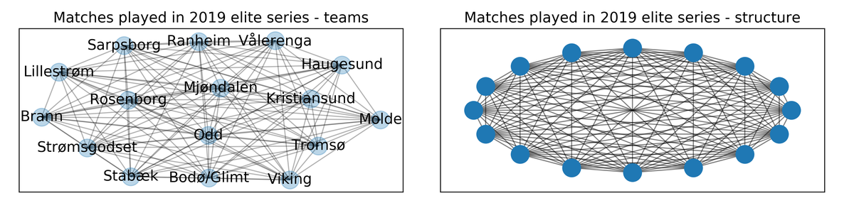
The training data contains matches in the elite series from 2016, 2017 and 2018. There are \(720\) matches and \(19\) teams in the data set. The test data consists of \(240\) matches from the 2019 elite series.

The data has beautiful structure. Every match pairs two teams; the home team and away team. Team skill combine with some amount of randomness and luck, giving us observations of goals scored.

It’s common in the literature to model goals by a Poisson distribution. This approach seems justified when we examine goals scored in the training data. The Poisson assumption fits the data well. Note that teams on average score more goals on their home turf.

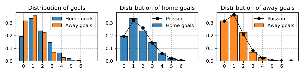
We denote home goals and away goals scored in a match by \(y^\text{h}\) and \(y^\text{a}\) respectively. The expected value of goals scored over all matches in the training data is:

A Bayesian model

A Bayesian model is a great approach for a structured problem such as this one, since:

• We are able to explicitly capture the rich structure in the data.
• The posterior predictive distribution gives a full probability of match outcomes.

Model structure

We assume that goals \(y\) are generated by a Poisson distribution \(p \left( y | \theta \right) = \theta^y \exp \left( -\theta \right) / y!\) with rate parameter \(\theta\). Every team has a latent attack and defence strength influencing \(\theta\). We model home advantage with a global parameter that is not team-specific. We also add an intercept (bias) to the model.

In an attempt to ease notation we do not explicitly index each match in the model description below. We use the parameter \(y^\text{h}\) to indicate goals scored by the home team, which is generated by a Poisson distribution with rate parameter \(\theta^\text{h}\). The meaning of \(\text{attack}_{i[\text{h}]}\) is “attack strength of team \(i\), which is the home team in the match.”

The generalized linear model uses a logarithmic link function with a Poisson distribution:

The attack and defence parameters are random variables with priors given by:

At this point the attack and defence parameters are not identifiable. In other words, they can be arbitrarily shifted since \(\text{attack}_{i} - \text{defence}_{i} = (\text{attack}_{i} + \alpha)- (\text{defence}_{i} + \alpha)\) for all values of \(\alpha\). To enforce identifiability we add soft constraints to the parameters.

Finally, the hyper-priors are given by:

That’s it! The structure of this simple model will likely do a good job on any team sport similar to football: handball, volleyball, basketball, etc.

Team strength

One of the virtues of Bayesian modeling is the ability to retrieve posterior distributions over model parameters. The attack strength and defence strength inferred by the model is shown below. The black dots indicate medians, while the bands indicate \(50 \, \%\) and \(90 \, \%\) of the probability.

There’s clearly a correlation between aggressive and defensive strength, but the model picks up some discrepancies too. The model is unsure about “Mjøndalen”, and with good reason; the team is not present in the training data. In this application the prior \(\text{attack}_i \sim \operatorname{Normal} \left( 0, \sigma_{\text{attack}} \right)\) combined with the identifiability constraint means that the posterior mode of attack and defence of “Mjøndalen” is set to \(0\). In reality, a new team entering the league is likely weaker than the rest. Perhaps a prior such as \(\operatorname{Normal} \left( -1/4, \sigma_{\text{attack}} \right)\) would be more appropriate. We do not pursue this approach here, since it won’t make a difference for most teams.

Out-of-sample predictions

By drawing thousands of samples from the posterior predictive distribution we can estimate the distribution over goal difference as well as the probability of a home win, a draw and a win for the visiting team. This process is shown for a single prediction on the test data in the figure below.

A posterior distribution over goal differences is easily obtained by computing the sum

Summing once again yields probabilities of outcomes. To compute the probability of a home win:

Applying the same process as above to \(12\) out-of-sample matches, we are able to generate probabilistic estimates over outcomes. This is shown in the figure below, where actual outcomes are shown in green.

Of course, the fact that “Strømsgodset” has a probability of \(51.5 \, \%\) of winning the match in the second row does not imply that they will always win. The model merely predicts that in approximately \(51\) out of \(100\) matches, “Strømsgodset” would win against “Bodø/Glimt”. In the actual match “Bodø/Glimt” won.

Modeling home team advantage on the team level

It might be the case that some teams perform disproportionately better at home. To investigate this, we replace the global parameter \(\text{home}\) with a team-specific parameter \(\text{home}_{i[\text{h}]}\) and model home advantage as

The figure below shows the posterior distribution of team-specific attack, defence and home advantage.

Recall that the training data consists of matches in the elite series from 2016, 2017 and 2018. We extend the data by adding every league that the teams played in. This introduces many more teams and matches to the training data set. The result is shown in the figure below.

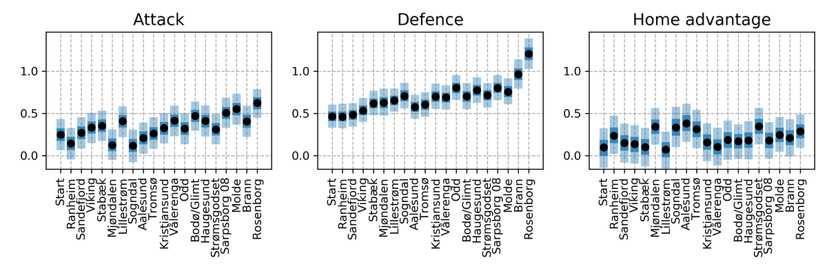
Notice the \(y\)-axis in the figure above; the teams all have high parameter values. This is because the identifiability constraints range over all teams in the training data, and the teams of interest (playing in the elite series) are better than average. The model is now more sure about “Mjøndalen”, since it is included in the training data set.

Unfortunately, neither modeling home advantage as team-dependent nor adding more data significantly improved the predictive power on the test data.

Extensions

While the model presented is simple, it correctly picks up team strengths that are in accordance with observed results. Many extensions are possible to enrich the model, some of which are:

• Players and management.   A team consists of players and management.   Information about the players that played each match and the management of the team might improve the model.   Even if predictive power is not improved, it would be interesting to infer player strengths directly from matches.
• Years or seasons.   Instead of explicitly modeling players, we can assume some variation from season to season due to player influx and outflux.   Adding this to the model might help model the uncertainty present in a future season.
• Model ensembles. There are many features that could help predict match outcomes, though some might be hard to fit into a Bayesian framework.   For instance, time since the last match, expert opinions, toughness of the previous match, weather conditions, media coverage, etc. might be viable.   A model ensemble consisting of a non-Bayesian and Bayesian model might increase predictive power.

Summary

Team sports can be modeled using a generalized linear model, where goals are assumed to be Poisson distributed. A Bayesian approach is excellent for this problem because it allows us to encode the structure of the data in the model, and because it yields a full posterior distribution. Modeling home advantage on the team level did not significantly improve predictive power, but there are many other extensions which might.

Notes and references

• “Bayesian hierarchical model for the prediction of football results” by Baio et al. uses the same basic model structure as the one introduced here.
• “A Bayesian inference approach for determining player abilities in soccer” by Whitaker et al. builds on the paper by Baio by introducing players to the mix.
• “Bayesian statistics meets sports: a comprehensive review” by Santos-Fernandez et al. reviews how sports such as football, basketball and baseball are modeled in 74 papers.