Suppose a government agency has a total budget of \(B\) dollars. The agency wants to allocate this budget to several projects. The projects are indexed by \(i\). Each project has a claim to a certain percentage of the budget, and \(d_i\) indicates the distribution of the total budget \(B\) over each individual project \(i\). The values \(d_i\) are relative numbers (percentages).

Let’s look at a simple example to concretize the problem.

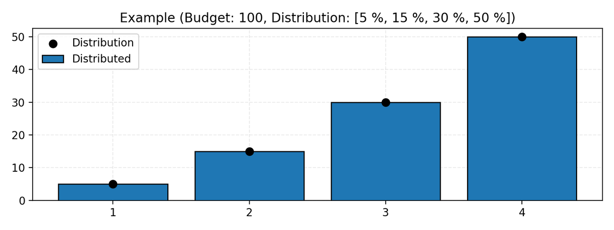
In the figure below, the total budget is \(B = 100\). Project 1 has a claim of \(d_i = 5 \%\) of the budget \(B\), project 2 has a claim of \(d_i = 15 \%\) of the budget \(B\), project 3 has a claim of \(d_i = 30 \%\) of the budget \(B\) and project 4 has a claim of \(d_i = 50 \%\) of the budget \(B\).

The solution is simple: project \(i\) gets allocated \(p_i \times B\).

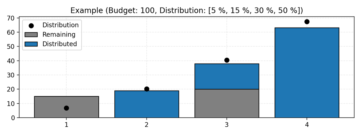
Now let us complicate the problem slightly. Each project may have remaining funds \(r_i \geq 0\), perhaps from the previous year. These funds cannot be re-allocated to a different project.

The figure below shows the same problem, but \(r_1 = 15\) and \(r_3 = 20\). Notice that the values \(d_i\), represented in the figure using black dots, do not sum to \(100\). This does not matter since they are relative sizes (percentages) and can be scaled however we like.

How can we allocate the budget \(B\), so each project ends up with an allocation that is, relatively, as close as possible to the desired distribution? We must take the remaining funds \(r_i\) into account. By relatively, I mean that it’s better if two projects that desire \(20\%\) and \(40\%\) end up with respectively \(10\%\) and \(20\%\) (half each), rather than e.g. minimizing the maximum difference so the projects get \(5\%\) and \(25\%\).

Solution by convex optimization

One way to solve the problem is to formulate it as a convex optimization problem and give it to a solver.

We scale the distribution \(p_i\) and introduce percentages \(p_i\):

Then we write a convex optimization problem that minimizes the relative error:

In vector notation, we minimize the quadratic form \(\left( \mathbf{r} + \mathbf{x} - \mathbf{p} \right)^T \operatorname{diag}(1/\mathbf{p}) \left( \mathbf{r} + \mathbf{x} - \mathbf{p} \right)\).

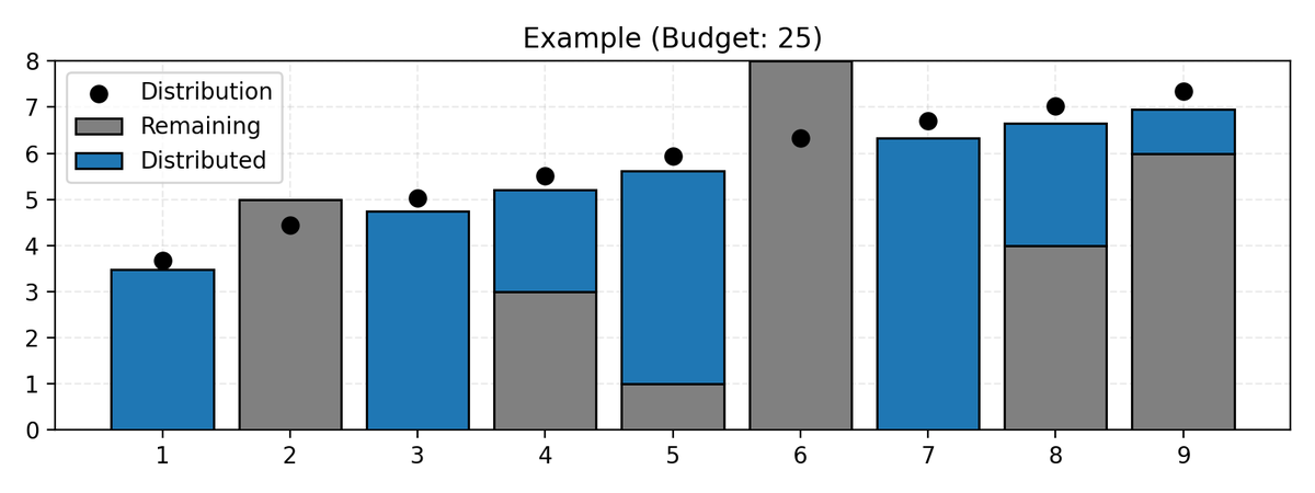
The solution to the problem instance above looks like this:

Here is the Python code implementing the model above, using CVXPY:

def allocate_cvxpy(distribution, remaining, budget):
    import cvxpy as cp

    total = np.sum(remaining) + budget  # Total that will be distributed
    percentage = total * (distribution / np.sum(distribution))

    # Set up problem
    x = cp.Variable(len(distribution))
    squares = cp.square((remaining + x - percentage)) / percentage
    objective = cp.Minimize(cp.sum(squares))
    constraints = [cp.sum(x) == budget,  # Must distribute everything
                   x >= 0]               # No negative numbers

    problem = cp.Problem(objective, constraints)
    problem.solve() # Solve using OSQP solver
    return np.abs(np.array(x.value)) # Take abs so solution is non-negative

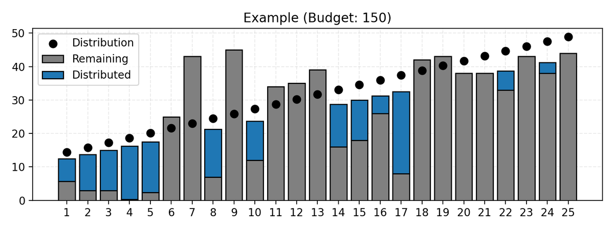
Here is another problem instance and its solution:

Solution by root-finding

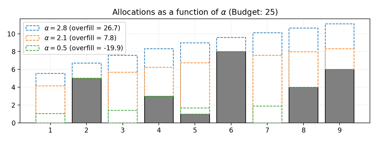
Instead of using a general convex optimization package, we can formulate the problem as root-finding. Given a factor \(\alpha\) that we use to scale the distribution \(d_i\), we can compute the overfill with respect to our budget \(B\) as

Since \(\text{overfill}(\alpha)\) is monotonically non-decreasing in \(\alpha\), and since when \(\text{overfill}(\alpha^{\star}) = 0\) when the budget \(B\) is used up, we can use a root-finding algorithm to find the optimal \(\alpha^{\star}\). In fact, it’s easy to see that \(\text{overfill}(\alpha)\) is convex.

Here is what the code might look like:

def allocate_rootfinding(distribution, remaining, budget):
    from scipy.optimize import root_scalar

    def overfill(alpha):
        """Multiplying the distribution by alpha, what is the overfill?"""
        return np.maximum(alpha * distribution - remaining, 0).sum() - budget

    # Compute an upper bound by placing everything in one project
    i = np.argmax(distribution)
    upper_bound = (remaining[i] + budget) / distribution[i] + 1

    # Search for the alpha which produces exactly 0 overfill
    result = root_scalar(overfill, method="brentq", bracket=[0, upper_bound])

    return np.maximum(result.root * distribution - remaining, 0)

Here’s a figure showing some values of \(\alpha\) and the overfill values, on the same problem instance that we looked at before.

Here is a final example:

Notes

• The problem is somewhat similar to the water-filling-algorithm, which is explained Example 5.2 in the book “Convex Optimization” by Boyd et al.
• On a random problem with a thousand projects, the convex optimization approach took 14.8 ms while the root-finding approach took 136 µs.